Comparison with the python-dro package

TLDR

A new toolbok appeared for general DRO. Their support for Wasserstein ambiguity sets is limited to certain specific models; SkWDRO is thus complementary to it. In the intersection of our two playgrounds, one can find (regularized) WDRO linear regressions. So we run a quick comparison notebook below. In short: both get similar accuracy performances, but SkWDRO often yields similar or better running times.

In December 2023, the library python-dro was released by a team of experts of Distributionally Robust Optimisation. It tackles a very wide range of ambiguity sets (for Maximum-Mean-Discrepancy, KL, etc). They propose both the Wasserstein ambiguity set as well as its Sinkhorn-regularized counterpart. The version 0.3.3 of their repository is limited to what follows:

• for WDRO: only for linear models, and for specific neural networks under \(W_\infty\) uncertainty (i.e. adversarial attacks, of the same flavor as so-called “fast-gradient-sign attacks”),

• for Sinkhorn-regularized-WDRO: only for linear models

This example notebook illustrates the use of the skwdro.linear_models.LinearRegression side to side with the (KL-regularized or not) version of WDRO implemented by the python-dro library. The aim is to illustrate the two libraries on the intersection of their application domains.

import timeit
import subprocess
import tqdm.auto as tqdm

import matplotlib.pyplot as plt
import numpy as np
import pandas as pd

from sklearn.datasets import make_regression
from sklearn.preprocessing import minmax_scale
from sklearn.model_selection import train_test_split
from sklearn.metrics import mean_squared_error
from sklearn.utils import check_X_y

from dro.linear_model.wasserstein_dro import WassersteinDRO
from dro.linear_model.sinkhorn_dro import SinkhornLinearDRO
from skwdro.linear_models import LinearRegression

Problem setup

# Total number of samples: chosen to be a bit prohibitive for SVM-like kernel methods (would deserve a separate analysis)
n = 512
# "Low"-dimensional setting to avoid this notebook to run for unreasonable amounts of time.
d = 4
n_train = int(np.floor(0.8 * n)) # Number of training samples: 80% of dataset
n_test = n - n_train # Number of test samples

# Generate some data
X, y, *_ = make_regression(n_samples=n, n_features=d, noise=50, random_state=0)
assert isinstance(X, np.ndarray)

# Normalize the data
X = minmax_scale(X, feature_range=(-1, 1))
y = minmax_scale(y, feature_range=(-1, 1))

# Split the data into training and test sets
X_train, X_test, y_train, y_test = train_test_split(X, y, train_size=n_train, test_size=n_test, random_state=0)
assert isinstance(X_train, np.ndarray)
assert isinstance(X_test, np.ndarray)

Some more words on the setup

For reproducibility, we make notice of the fact that the results obtained bellow are obtained for a low number of runs, in order to reduce the time needed to launch them.

Note

All benchmarks presented are run on CPU. GPU experiments are not yet available.

Warning

This small script only works with unix-compatible shells/distributions.

These are the exact machine details:

for title, command in [
    ('System spec.:', ['uname', '-mrs']),
    ('Memory (RAM):', ['grep', 'MemTotal', '/proc/meminfo']),
    ('CPU cores:', ['grep', 'model name', '/proc/cpuinfo']),
    ('CPU infos:', ['lshw', '-class', 'cpu', '-sanitize', '-notime'])
]:
    print(title)
    _output = subprocess.run(command, stdout=subprocess.PIPE).stdout.decode('utf-8')
    if 'CPU' in title:
        print(*_output.split('model name\t: '))
    else:
        print(_output)

System spec.:
Linux 6.8.0-90-generic x86_64

Memory (RAM):
MemTotal:       32464404 kB

CPU cores:
 13th Gen Intel(R) Core(TM) i7-13800H
 13th Gen Intel(R) Core(TM) i7-13800H
 13th Gen Intel(R) Core(TM) i7-13800H
 13th Gen Intel(R) Core(TM) i7-13800H
 13th Gen Intel(R) Core(TM) i7-13800H
 13th Gen Intel(R) Core(TM) i7-13800H
 13th Gen Intel(R) Core(TM) i7-13800H
 13th Gen Intel(R) Core(TM) i7-13800H
 13th Gen Intel(R) Core(TM) i7-13800H
 13th Gen Intel(R) Core(TM) i7-13800H
 13th Gen Intel(R) Core(TM) i7-13800H
 13th Gen Intel(R) Core(TM) i7-13800H
 13th Gen Intel(R) Core(TM) i7-13800H
 13th Gen Intel(R) Core(TM) i7-13800H
 13th Gen Intel(R) Core(TM) i7-13800H
 13th Gen Intel(R) Core(TM) i7-13800H
 13th Gen Intel(R) Core(TM) i7-13800H
 13th Gen Intel(R) Core(TM) i7-13800H
 13th Gen Intel(R) Core(TM) i7-13800H
 13th Gen Intel(R) Core(TM) i7-13800H

CPU infos:
  *-cpu
       product: 13th Gen Intel(R) Core(TM) i7-13800H
       vendor: Intel Corp.
       physical id: 1
       bus info: cpu@0
       version: 6.186.2
       size: 1143MHz
       capacity: 5GHz
       width: 64 bits
       capabilities: fpu fpu_exception wp vme de pse tsc msr pae mce cx8 apic sep mtrr pge mca cmov pat pse36 clflush dts acpi mmx fxsr sse sse2 ss ht tm pbe syscall nx pdpe1gb rdtscp x86-64 constant_tsc art arch_perfmon pebs bts rep_good nopl xtopology nonstop_tsc cpuid aperfmperf tsc_known_freq pni pclmulqdq dtes64 monitor ds_cpl vmx smx est tm2 ssse3 sdbg fma cx16 xtpr pdcm pcid sse4_1 sse4_2 x2apic movbe popcnt tsc_deadline_timer aes xsave avx f16c rdrand lahf_lm abm 3dnowprefetch cpuid_fault epb ssbd ibrs ibpb stibp ibrs_enhanced tpr_shadow flexpriority ept vpid ept_ad fsgsbase tsc_adjust bmi1 avx2 smep bmi2 erms invpcid rdseed adx smap clflushopt clwb intel_pt sha_ni xsaveopt xsavec xgetbv1 xsaves split_lock_detect user_shstk avx_vnni dtherm ida arat pln pts hwp hwp_notify hwp_act_window hwp_epp hwp_pkg_req hfi vnmi umip pku ospke waitpkg gfni vaes vpclmulqdq tme rdpid movdiri movdir64b fsrm md_clear serialize pconfig arch_lbr ibt flush_l1d arch_capabilities ibpb_exit_to_user cpufreq
       configuration: microcode=16681

WDRO linear regression

Bellow we define multiple models for the robust optimization of a linear regression problem (OLS):

• the non-regularized original WDRO formulation, cast as a convex optimization problem for the 2-norm squared (i.e. \(W_2\) measure transport cost, for the Mahalanobis distance),

• the regularized Sinkhorn-Wasserstein distance according to the two similar approaches of Gao et al. [2] and Azizian et al. [1] with regard to the way the problem is dualized, both in the same hyperparameter settings.

We set a few of the hyperparameters: the distance used for the ground-cost is the norm (squared) with unit metric tensor ( implying also an isotropic covariance matrix for the sampler), and no target switches allowed. The variance of the sampler is fixed, as well as the regularization parameter.

rhos = [1e-6, 1e-3, 1e-1]
SIGMA = 1e-2
EPSILON_REGULARISATION = 1e-1

def fit_wdro_from_dro(rho: float):
    estimator = WassersteinDRO(
        input_dim=d,
        solver='SCS',
        model_type='ols'
    )
    estimator.update({
        'cost_matrix': np.eye(d),
        'eps': rho**2,
        'p': 2,
        'kappa': 'inf'
    })
    estimator.fit(*check_X_y(X_train, y_train))
    return estimator

def fit_skwdro_from_dro(rho: float):
    estimator = SinkhornLinearDRO(
        input_dim=d,
        fit_intercept=True,
        max_iter=5_000,
        reg_param=EPSILON_REGULARISATION,
        model_type='ols'
    )
    estimator.update({
        'cost_matrix': np.eye(d),
        'eps': rho**2,
        'p': 2,
        'kappa': 'inf'
    })
    estimator.fit(*check_X_y(X_train, y_train))
    return estimator

def fit_wdro_from_skwdro(rho: float):
    estimator = LinearRegression(
        solver='dedicated',
        rho=rho,
        fit_intercept=True
    )
    estimator.fit(X_train, y_train)
    return estimator

def fit_skwdro_from_skwdro(rho: float):
    estimator = LinearRegression(
        rho=rho,
        sampler_reg=SIGMA,
        learning_rate=1e-3,
        n_iter=5_000,
        solver_reg=EPSILON_REGULARISATION,
        fit_intercept=True
    )
    estimator.fit(X_train, y_train)
    return estimator

estimators_funcs = [
    fit_wdro_from_dro,
    fit_skwdro_from_dro,
    fit_wdro_from_skwdro,
    fit_skwdro_from_skwdro
]

Evaluation

all_train_errors = []
all_test_errors = []
all_timers = []
method_names = [
    'WDRO (p-dro)',
    'Sk-WDRO (p-dro)',
    'WDRO (skwdro)',
    'Sk-WDRO (skwdro)'
]

for rho in tqdm.tqdm(rhos, desc='Radii', position=0, leave=True):
    train_errors = []
    test_errors = []
    timers = []

    for fitter in tqdm.tqdm(estimators_funcs, desc='Method-score', leave=False, position=1):
        estimator = fitter(rho)
        train_errors.append(mean_squared_error(y_train, estimator.predict(X_train)))
        test_errors.append(mean_squared_error(y_test, estimator.predict(X_test)))

    all_train_errors.append(train_errors)
    all_test_errors.append(test_errors)

    for fn in [
        'fit_wdro_from_dro',
        'fit_skwdro_from_dro',
        'fit_wdro_from_skwdro',
        'fit_skwdro_from_skwdro'
    ]:
        timers.append(timeit.timeit(fn+'(rho)', globals=globals(), number=3))

    all_timers.append(timers)

Radii:   0%|          | 0/3 [00:00<?, ?it/s]

Method-score:   0%|          | 0/4 [00:00<?, ?it/s]

Method-score:  50%|█████     | 2/4 [00:44<00:44, 22.38s/it]

Method-score: 100%|██████████| 4/4 [01:10<00:00, 16.66s/it]


Radii:  33%|███▎      | 1/3 [04:37<09:14, 277.44s/it]

Method-score:   0%|          | 0/4 [00:00<?, ?it/s]

Method-score:  50%|█████     | 2/4 [00:44<00:44, 22.03s/it]

Method-score: 100%|██████████| 4/4 [01:08<00:00, 16.16s/it]


Radii:  67%|██████▋   | 2/3 [09:11<04:34, 274.99s/it]

Method-score:   0%|          | 0/4 [00:00<?, ?it/s]

Method-score:  50%|█████     | 2/4 [00:43<00:43, 21.80s/it]

Method-score: 100%|██████████| 4/4 [01:08<00:00, 16.36s/it]


Radii: 100%|██████████| 3/3 [13:42<00:00, 273.18s/it]
Radii: 100%|██████████| 3/3 [13:42<00:00, 274.04s/it]

Plotting

# ----------------------------------------------------------------------
# Generic comparison plotting helper
# Author: chat-gpt
# Don't expect type stability
# ----------------------------------------------------------------------

def plot_library_comparison(
    df: pd.DataFrame,
    methods_python_dro: list,
    methods_skwdro: list,
    y_key: str,
    title: str,
    fname: str,
    cmap_python='viridis',
    cmap_skwdro='magma'
):
    """
    df: dataframe with columns ['rho', 'method', y_key]
    methods_python_dro: methods to plot with square markers + dashed line
    methods_skwdro: methods to plot with filled circle markers + solid line
    y_key: 'test_error' or 'time'
    """

    plt.figure(figsize=(10, 5))
    ax = plt.gca()

    # Create numeric x-axis from categorical rhos
    x_vals = np.arange(df['rho'].nunique())
    rho_labels = sorted(df['rho'].unique(), key=lambda x: int(x[5:-2]))  # sort by exponent
    rho_to_x = {rho: i for i, rho in enumerate(rho_labels)}

    # Build colormaps
    cmap_py = plt.get_cmap(cmap_python, len(methods_python_dro))
    cmap_sk = plt.get_cmap(cmap_skwdro, len(methods_skwdro))

    # Python-DRO models → dashed lines + empty squares
    for k, method in enumerate(methods_python_dro):
        sub = df[df['method'] == method]
        xs = [rho_to_x[r] for r in sub['rho']]
        ys = sub[y_key].values
        ax.plot(xs, ys,
                linestyle='--',
                marker='s',
                markersize=10,
                markerfacecolor='none',
                markeredgecolor=cmap_py(k),
                color=cmap_py(k),
                linewidth=2,
                label=f"{method} (python-dro)")

    # SkWDRO models → solid lines + filled circles
    for k, method in enumerate(methods_skwdro):
        sub = df[df['method'] == method]
        xs = [rho_to_x[r] for r in sub['rho']]
        ys = sub[y_key].values
        ax.plot(xs, ys,
                linestyle='-',
                marker='o',
                markersize=9,
                markerfacecolor=cmap_sk(k),
                markeredgecolor=cmap_sk(k),
                color=cmap_sk(k),
                linewidth=2,
                label=f"{method} (skwdro)")

    ax.set_xticks(x_vals)
    ax.set_xticklabels(rho_labels)
    ax.set_yscale('log')
    ax.set_xlabel("ρ (Wasserstein radius)")
    ax.set_ylabel(y_key.replace('_', ' ').title())
    ax.set_title(title)
    ax.legend()
    return ax

def _rho_formatter(rho: float) -> str:
    return "$10^{" + f"{int(np.log10(rho))}" + "}$"

# Build pandas DataFrames for seaborn (rho treated as categorical)
train_df = pd.DataFrame([
    {'rho': _rho_formatter(rhos[i]), 'method': method_names[j], 'train_error': all_train_errors[i][j]}
        for i in range(len(rhos)) for j in range(len(method_names))
])

test_df = pd.DataFrame([
    {'rho': _rho_formatter(rhos[i]), 'method': method_names[j], 'test_error': all_test_errors[i][j]}
        for i in range(len(rhos)) for j in range(len(method_names))
])

time_df = pd.DataFrame([
    {'rho': _rho_formatter(rhos[i]), 'method': method_names[j], 'time': all_timers[i][j]}
        for i in range(len(rhos)) for j in range(len(method_names))
])

WDRO comparison plots

We first propose a plot comparing disciplined WDRO implementations across libraries. It compares the test losses for the two methods, evaluated as the ERM (with mean-squared error), and the wall-clock running times.

wdro_methods = ['WDRO (p-dro)', 'WDRO (skwdro)']
wdro_test = test_df[test_df['method'].isin(wdro_methods)]
wdro_time = time_df[test_df['method'].isin(wdro_methods)]
assert isinstance(wdro_test, pd.DataFrame)
assert isinstance(wdro_time, pd.DataFrame)

Test loss plot

plot_library_comparison(
    df=wdro_test,
    methods_python_dro=['WDRO (p-dro)'],
    methods_skwdro=['WDRO (skwdro)'],
    y_key='test_error',
    title='WDRO Test Errors Across Libraries',
    fname='/tmp/wdro_test_errors.png'
)

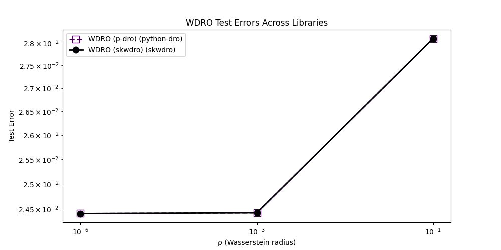
<Axes: title={'center': 'WDRO Test Errors Across Libraries'}, xlabel='ρ (Wasserstein radius)', ylabel='Test Error'>

We see that the two libraries are relatively similar, especially for small Wasserstein radii, which is to be expected considering the similarity between the implementations, based on the standard techniques of [3] and [4].

Timing plot

plot_library_comparison(
    df=wdro_time,
    methods_python_dro=['WDRO (p-dro)'],
    methods_skwdro=['WDRO (skwdro)'],
    y_key='time',
    title='WDRO Timing Across Libraries',
    fname='/tmp/wdro_timing.png'
)

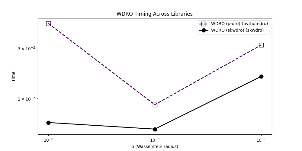
<Axes: title={'center': 'WDRO Timing Across Libraries'}, xlabel='ρ (Wasserstein radius)', ylabel='Time'>

The running times of the two libraries are usually comparable, even though it seems like the implementation in SkWDRO seems faster in some setting.

SK-WDRO comparison plots

Here is another set of plots comparing regularized WDRO implementations, for the two libraries, both relying under the hood on PyTorch.

Let’s compare Sinkhorn-based WDRO models from both libraries

sk_methods = ['Sk-WDRO (p-dro)', 'Sk-WDRO (skwdro)']
sk_test = test_df[test_df['method'].isin(sk_methods)]
sk_time = time_df[test_df['method'].isin(sk_methods)]
assert isinstance(sk_test, pd.DataFrame)
assert isinstance(sk_time, pd.DataFrame)

Test loss plot

plot_library_comparison(
    df=sk_test,
    methods_python_dro=['Sk-WDRO (p-dro)'],
    methods_skwdro=['Sk-WDRO (skwdro)'],
    y_key='test_error',
    title='Sk-WDRO Test Errors Across Libraries',
    fname='/tmp/skwdro_test_errors.png'
)

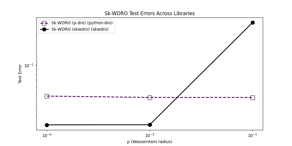
<Axes: title={'center': 'Sk-WDRO Test Errors Across Libraries'}, xlabel='ρ (Wasserstein radius)', ylabel='Test Error'>

Timing plot

plot_library_comparison(
    df=sk_time,
    methods_python_dro=['Sk-WDRO (p-dro)'],
    methods_skwdro=['Sk-WDRO (skwdro)'],
    y_key='time',
    title='Sk-WDRO Timing Across Libraries',
    fname='/tmp/skwdro_timing.png'
)

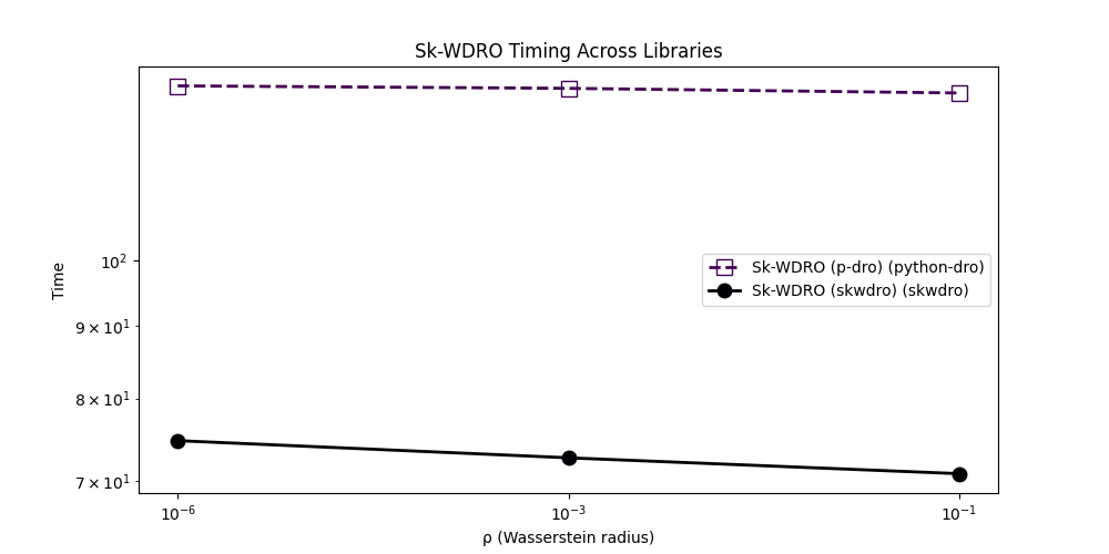
<Axes: title={'center': 'Sk-WDRO Timing Across Libraries'}, xlabel='ρ (Wasserstein radius)', ylabel='Time'>

The speed of SkWDRO is usualy higher in this low dimensional setting with a medium-sized dataset. Other experiments could be run to show more balanced results with fewer samples (e.g. we obtained closer timings with \(n=100\)), or some times more drastic difference of running time performance.

For the test accuracy though, it seems to depend heavily on the chosen robustness radius: for smaller radii SkWDRO is more performant while the technique from [2] is more suited for higher radii. We have the intuition that this comes from the implementation in python-dro which fixes the dual parameter \(\lambda\), removing the need to optimize it. In exchange, this forces the user to pick a good starting value for it. We invite curious readers to tune it by hand for their code in order to see better and more radius-agnostic convergence properties.

Tackling non-linear models

To highlight the difference between SkWDRO and python-dro, we argue that our library’s approach focuses on large parameters space models like neural networks that are not implementable in python-dro nor in other frameworks. This is illustrated in other tutorials in this documentation.

Neural nets on simple examples

You can first try our library on simpler low-dimensional examples that are tractable enough for obtaining quick and easy visual cues. This is illustrated in more details in the moons dataset example, in a simple two dimensional setting with a non-linearly-separable dataset.

Neural net on more difficult datasets

This approach scales to higher-dimensional settings, at the expense of computation time. We showcase this on the iWildsCam dataset, in a separate documentation page.

References

[1]

Azizian, Iutzeler, and Malick: Regularization for Wasserstein Distributionally Robust Optimization, COCV, 2023

[2] (1,2)

Wang, Gao, and Xie: Sinkhorn Distributionally Robust Optimization, arXiv (2109.11926), 2023

[3]

Shafieezadeh-Abadeh, Kuhn, and Esfahani: Regularization via Mass Transportation, JMLR, 2019

[4]

Esfahani and Kuhn: Data-Driven Distributionally Robust Optimization Using the Wasserstein Metric: Performance Guarentees and Tractable Reformulations, Mathematical Programming, 2017