Why SkWDRO?#
Theory
Let us now present the ideas in this library.
You may prefer to read the previous tutorial on WDRO to understand better this part.
About the library#
As we will see bellow, the WDRO approach has some issues that make it difficult to implement for arbitrary loss functions.
Of course, if one has a very structured problem (say linear by part, \(c\)-concave, etc), they should by all means turn to WDRO or other DRO approaches via \(\phi\)-divergences before trying our approach in SkWDRO.
But, when strugling with less structured cases, like deep learning applications with complicated distribution shifts, SkWDRO remains as one of the rare tractable approaches to (distributional) robustness.
Thus, the library aims at providing easy-to-use interfaces in PyTorch (a Python library to perform machine learning on various backends) to do some minimal changes to your model in order to robustify it.
Pronouncing its name#
The idea of SkWDRO comes from a modification of WDRO (see the previous tutorial on the topic).
The prefix Sk is added as a pun mixing “Sinkhorn”, the name of the entropic regularization term we use, and “scikit”(-learn) which is the python library for some of the out-of-the-box (Sk-)WDRO examples we coded, as a layer of abstraction.
In the dev team, we ended up pronouncing it by spelling the six letters, but we still believe it sounds great phonetically with a slight french accent as well (s-qu-ou-drô/secoue-drô, pun intended).
What is wrong with WDRO?#
Recall the general “tractable” formula for WDRO:
While in small dimension \(d\) and with a concave loss \(L_\theta\) (or concave \(c\)-transformed loss) this supremum expression in (1) might seem tractable at first, it becomes prohibtively complicated in any other setting: the optimality conditions may be non-obvious, spurious maxima are to be expected in the non-concave cases, and algorithms to solve the optimality conditions are not guarenteed to reach a good convergence. One will also need to leverage some fashion of the implicit function theorem to sort out the dependency between the optimal \(\zeta^*\) and the parameters \(\theta\) in order to perform descent algorithms on the latter.
Then what can we do about it?#
A great solution to this problem is offered in [1], following [3]. It relies on a regularization of the optimal transport problem, by adding an entropic term \(- \varepsilon\mathcal{D}_{KL}(\pi\|\pi_0)\) to the Wasserstein-DRO problem.
Note
Notice the presence of a new hyperparameter \(\pi_0\), that we call the “reference measure”. It encodes the beliefs that we have about the problem studied, related to the optimal transport plan. Its first marginal should be \(\hat{\mathbb{P}}^N\) in order for the “true” optimal transport plan from WDRO to remain absolutely continuous with respect to it, as this is an important requirement for the regularization term to be finite.
Smoothing and DRO#
This technique “smoothes” the notion of neighborhood introduced by the Wasserstein transport cost. Such smoothing has already been used for the computation of the transport cost itself, e.g. in the POT library, for its great numerical advantages. The motivation here is similar and allows a tractable reformulation.
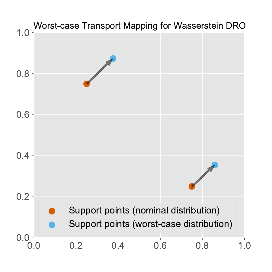
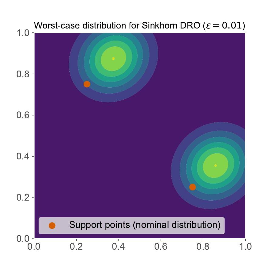
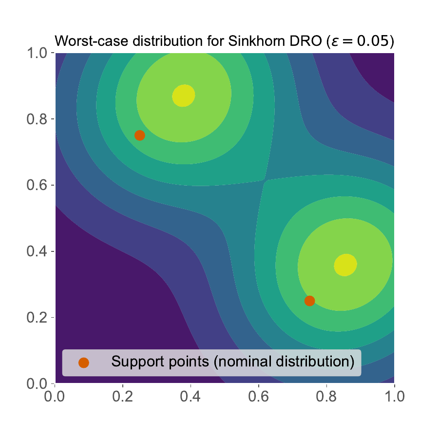
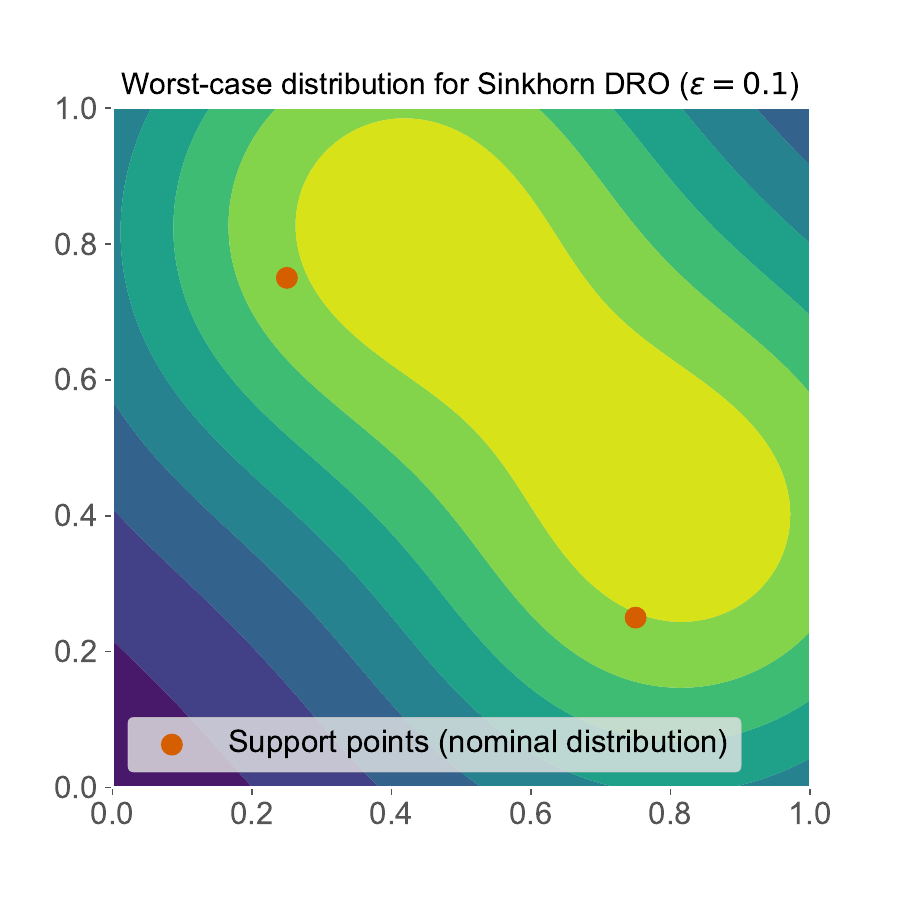
Bellow is a graphical representation taken from [3], showcasing for some loss function the optimal transport plan computed analytically, for some reference distribution admitting a density function (\(\pi^*\ll\pi_0\)). The red points correspond to \(\hat{\mathbb{P}}^N\). Notice how WDRO sends Diracs to Diracs, while its Sinkhorn regularization remains absolutely continuous with respect to \(\pi_0\).
|
|
|
|
|---|---|---|---|
Optimal \(\pi^*\) for WDRO |
Optimal \(\pi^*\) for \(\varepsilon=0.01\) |
Optimal \(\pi^*\) for \(\varepsilon=0.05\) |
Optimal \(\pi^*\) for \(\varepsilon=0.1\) |
Reformulation of the DRO problem with Sinkhorn-regularization of WDRO#
As [1] explains, the regularization term can either be added to the constraint term \(W_c(\hat{\mathbb{P}}^N, \mathbb{Q})\) to soften the neighborhood’s contours (close to what is proposed by [3]), or to the objective function directly \(\sup_{\pi\in\Pi(\hat{\mathbb{P}}^N, \cdot)}\mathbb{E}_{(\xi, \zeta)\sim\pi}\left[L_\theta(\zeta)\right] - \varepsilon\mathcal{D}_{KL}(\pi\|\pi_0)\).
There is no a priori theoretical reason to prefer one over the other, and [1] studies the combination of both. So in this library, for purely computational reasons, we prefer to perform the regularization directly in the objective because the dual formula that then emerges has less dependency on the dual parameter \(\lambda\) (thus avoiding some instablities):
Advantages and drawebacks of skwdro#
Here is sumarized what we won and lost through the regularization process.
/ |
Pros |
Cons |
|
|---|---|---|---|
\(\sup_{\zeta}\, L_{\theta}(\zeta)\;-\;\lambda\, c(\zeta,\xi)\) |
|
|
|
\(\varepsilon \log \mathbb{E}_{\zeta \sim \mathcal{N}(\xi,\sigma^2I)}\!\left[ e^{\left(L_{\theta}(\zeta)-\lambda\, c(\zeta,\xi)\right)/\varepsilon} \right]\) |
|
|
|
If the problem at hand benefits most from WDRO, a lot of good technical solutions should be found in e.g. the python-dro library. But in most cases, its application will not be directly possible: you shoud then turn to our library to leverage (2).
The smoothness of the “log-average-exponential” (i.e. log-sum-exp) expression in (2) is its main selling point: you can now plug it in you favorite SGD algorithm to get a solution, skipping theoretical work.
One of the main goals of the library is to offer the estimation of (2) on a plater, battery-included: the loss is differentiable by autodiff capabilities in order to plug it in your usual descent algotithm and some freedom is left for you to tune it through the PyTorch library.
Thus we advise readers to take a good look at the PyTorch interface tutorial to learn how to use the interfaces.
Next#
Tutorial on how to use pre-implemented examples with their scikit-learn interface.
Tutorial on how to robustify your model easily with the pytorch wrappers.
More details about the exposed API.