Illustration on iWildsCam#
This short page aims at
illustrating the use of SkWDRO to robustify the performances of a Neural
Network on a real dataset: iWildsCam.
The dataset#
The iWildsCam dataset[2] is composed of images of animals from various places on earth. They are labeled with their specie title among 60 possible labels, as well as a location on earth. The dataset is then split in such a way that the training/validation set contains images from a fixed set of locations, and the test set contains images from other locations, absent from the training set.
This split of the dataset is an example of a distribution shift. Indeed the testing set contains visual features that are absent of the training set for a given animal, and hence cannot be seen by the machine learning model used. So this model must accomodate for this shift during its training in order to obtain good test results.
Methodology#
The data receives a pre-treatement as described in [1], using their trained neural network to provide a fix set of pretrained features that must be classified. As described in their paper, those pretrained features come from a Resnet50 network pretrained on Imagenet.
Both a multiclass logistic regression classifier and a shallow (two-layers)
neural network are tested.
They are fit for a regularized Wasserstein ambiguity set of type \(W_2\),
measured as the WDRO dual objective described in this tutorial,
for the Euclidean metric squared as ground cost, without allowing label switches.
The dual variable \(\lambda\) is optimized together with the parameters of the
neural network, with the Adam optimisation algorithm, and we discuss its impact
on the procedure below.
The ambiguity set’s radius \(\rho\) is set to a range of pre-defined values
\(\{10^{\{-6\dots -2\}}, 0\}\) that we compare by linking it to the color codes of the
curves below.
The ERM optimisation procedure is shown as reference in black.
We report those results below, showing how the optimisation procedure manages to
achieve good accuracies in multiple hyperparameters setting.
Results#
We show the results obtained from run scripts one may find in our supplementary experiments repository, running the following command:
$ # Optional: relaunch the experiments
$ # uv run optim_script.v2.py -s 0.001 -is on -l -m train
$ # Plot results
$ uv run optim_script.v2.py -s 0.001 -is on -l -m plot_acc
Warning
As a disclaimer: this part of the code is not per se part of the
SkWDRO library, hence it does not abide to its quality standards. It is
meant as a research script to investigate this specific dataset, and did not
receive the same care as the library itself.
You may of course play with the hyperparameters available. By default, the
options let you train a shallow network with one hidden layer (of 64 neurons).
You can change the training hyperparameters, but you will need to dive into the
code to change more subtle settings like the architecture. Still, a linear model
(with the -c flag) is available.
Please refer to the output of the help section to get more details:
$ uv run optim_script.v2.py --help
The neural net example#
The training outcomes for the neural network is as follows:
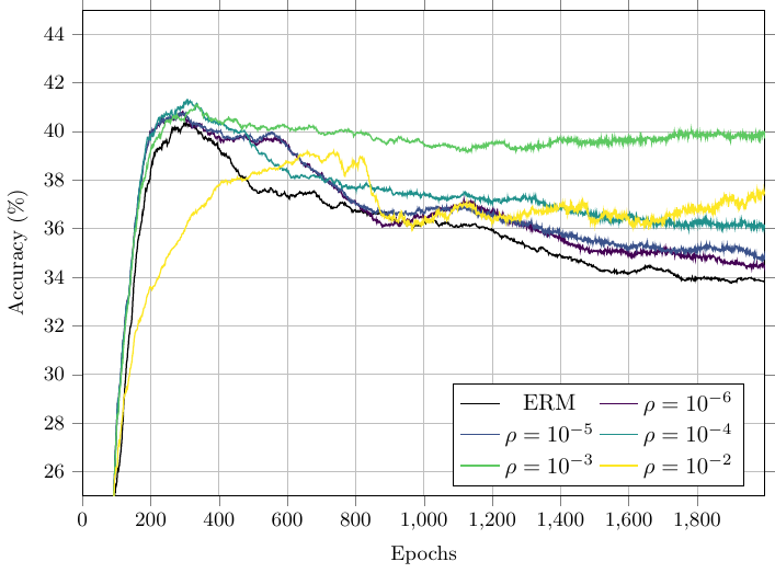
Notice how the overfitting behaviour changes substantially with the robustness radius \(\rho\).
For small values of \(\rho\), the accuracy raises in the first hundred iterations, and then goes down as the training procedure overfits the training set.
In contrast, for higher values of \(\rho\), the test performances are better and increase more steadily. From 300 epochs the performance does not degrade along training.
As a side-result, one may study the results of the \(\lambda\) optimisation depending on the chosen radius, and how much it changes. This way we may deduce how much importance we give to its optimisation (recall the experiments on lambda optimisation landscape).
$ uv run optim_script.v2.py -s 0.001 -is on -l -m tb_lam
Rho              | Lmin          | Lmax   | ratio
-       -       -       -
ρ=1.0e-06        | 109672        | 109752 | 1.00
ρ=1.0e-05        | 10975         | 11054  | 1.01
ρ=1.0e-04        | 1098          | 1180   | 1.08
ρ=1.0e-03        | 110           | 188    | 1.71
ρ=1.0e-02        | 11            | 102    | 9.32
-       -       -       -