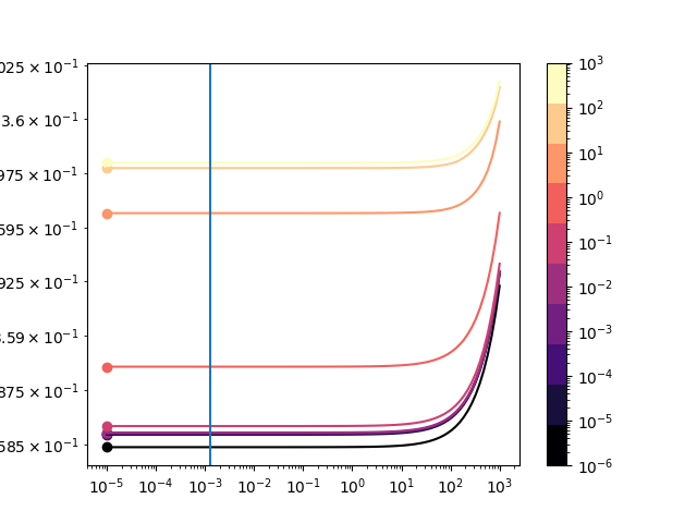
Understanding the landscape of the lambda optimisation

We use skwdro.torch.robustify to fit a linear classification model, then study at fixed parameters \(\theta\) the value of the robust loss for various values of \(\lambda\) the dual parameter..

import numpy as np

from sklearn.datasets import make_blobs

from skwdro.torch import robustify
from skwdro.linear_models._logistic_regression import BiDiffSoftMarginLoss
from sklearn.linear_model import LogisticRegression

import torch as pt
import torch.nn as nn

import matplotlib as mpl
import matplotlib.pyplot as plt
from matplotlib.cm import ScalarMappable

from matplotlib.colors import LogNorm
from tqdm import tqdm


# Helper function
def my_cm(ncolors=1000):
    return mpl.colormaps['magma'].resampled(ncolors)

device = 'cpu'

This is the function that computes the dual loss for a fixed model (i.e. fixed parameters \(\theta\)), for input \(\lambda\) value.

@pt.no_grad()
def fwd(model, l, X, y):
    model._lam = pt.nn.Parameter(pt.tensor(l).to(X))
    return model(X, y).detach().cpu().numpy()

Setup

We set a small number of samples \(\{\xi_i\}_{i\le N}\), and create a simple 2-blobs classification dataset

n = 30 # Total number of samples

sdevs = (1, 5)

# Fix centers for blobs dataset
pos = 4
centers = [np.array([-pos,-pos]), np.array([pos,pos])]

# Create datasets with variance that is shifted at test time
X_train, y_train = make_blobs(n_samples=n, centers=centers, cluster_std=sdevs) # type: ignore

WDRO classifier

We build a classifier and plot its SkWDRO-loss as a function of lambda (unoptimized). Its parameters are set to the ERM solution, i.e.

\[\theta_0 := {\min_\theta}^{-1}\frac{1}{N}\sum_{i=1}^N L_\theta(\xi_i)\]

# Rho is chosen small enough for the curves to be readable
rho = 1e-3

# Enthropic regularization: test various ones (10 different choices).
regs = np.logspace(-6, 3, base=10, num=10)[::-1]

# Kappa: weight of label shift
kappa = 100000

# Cost:
# t: torch backend
# NLC: norm cost that takes labels into account
# 2 2 : squared 2-norm
# kappa: weight of label shift
cost = f"t-NLC-2-2-{kappa}"

erm_model = LogisticRegression().fit(X_train, y_train)
erm_params = (erm_model.coef_, erm_model.intercept_)

SkWDRO-defined classifier’s data needs to be torch tensor objects, so we cast it from numpy.

Note

One must verify that the labels y have a (N, 1) shape

The ERM weights are then copied

X_train, y_train = pt.from_numpy(X_train), pt.from_numpy(y_train).double().unsqueeze(-1)

loss = BiDiffSoftMarginLoss(reduction='none')
linear_model = nn.Linear(2, 1, bias=True)
linear_model.weight = pt.nn.Parameter(pt.from_numpy(erm_params[0]))
linear_model.bias = pt.nn.Parameter(pt.from_numpy(erm_params[1]))
linear_model = linear_model.to(X_train)

The 1-WDRO loss (without Sinkhorn regularization) is:

\[\frac{1}{N}\sum_{i=1}^NL_\theta(\xi_i) + \rho\|\theta\|_*\]

For the approximate classifiers, we pick various regularization coefficients \(\{\varepsilon_i\}_{i\le 10}\)

wdro_loss = loss(
    linear_model(X_train), y_train
).mean() + rho * pt.linalg.norm(linear_model.weight.flatten())
classifiers_collection = [
    robustify(
        loss,
        linear_model,
        pt.tensor(rho).to(X_train),
        X_train,
        y_train,
        cost_spec=cost,
        epsilon=eps,
        n_samples=100
    ).to(X_train) for eps in regs
]

Make plot

fig, ax = plt.subplots()
test_ls = np.logspace(-5, 3, base=10, num=100)
ls_track = []

it = tqdm(classifiers_collection)
cmap = my_cm(len(it))

for i, classifier in enumerate(it):
    ls = [fwd(classifier, l, X_train, y_train) for l in test_ls]
    ls_track.append(ls)
    plt.loglog(test_ls, np.array(ls), label=f"$\\varepsilon={classifier.epsilon.cpu().item():.0e}$", c=cmap(i))
    plt.scatter([test_ls[np.argmin(ls)]], [np.min(ls)], color=cmap(i), label=f'$\\lambda_{i}^*$')
plt.axvline(rho * pt.linalg.norm(linear_model.weight.flatten()).detach().item(), label=r'$\lambda=\rho\|\theta\|_2$')

plt.colorbar(ScalarMappable(cmap=cmap, norm=LogNorm(vmin=regs.min(), vmax=regs.max())), ax=ax)
plt.show()

  0%|          | 0/10 [00:00<?, ?it/s]
 10%|█         | 1/10 [00:00<00:02,  3.32it/s]
 20%|██        | 2/10 [00:00<00:02,  3.77it/s]
 30%|███       | 3/10 [00:00<00:01,  3.95it/s]
 40%|████      | 4/10 [00:01<00:01,  4.04it/s]
 50%|█████     | 5/10 [00:01<00:01,  4.08it/s]
 60%|██████    | 6/10 [00:01<00:00,  4.12it/s]
 70%|███████   | 7/10 [00:01<00:00,  4.12it/s]
 80%|████████  | 8/10 [00:01<00:00,  4.10it/s]
 90%|█████████ | 9/10 [00:02<00:00,  4.12it/s]
100%|██████████| 10/10 [00:02<00:00,  4.14it/s]
100%|██████████| 10/10 [00:02<00:00,  4.05it/s]

Optionally save the data

Save data

np.savez_compressed(
    "lambda_stiff.npz",
    l=ls_track,
    r=rho * pt.linalg.norm(linear_model.weight.flatten()).detach().item(),
    erm=loss(linear_model(X_train), y_train).mean().detach().item()
)