skwdro.linear_models.LinearRegression

class skwdro.linear_models.LinearRegression(rho=0.01, l2_reg=0.0, fit_intercept=True, cost='t-NLC-2-2', solver='entropic_torch', solver_reg=None, sampler_reg=None, n_zeta_samples: int = 10, random_state: int = 0, opt_cond: ~skwdro.solvers.optim_cond.OptCondTorch | None = <skwdro.solvers.optim_cond.OptCondTorch object>)[source]

A Wasserstein Distributionally Robust linear regression.

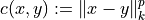
The cost function is

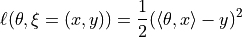
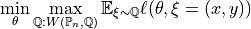
$\ell(\theta,\xi=(x,y)) = \frac{1}{2}(\langle \theta,x \rangle - y)^2$

The WDRO problem solved at fitting is

$\min_{\theta} \max_{\mathbb{Q} : W(\mathbb{P}_n,\mathbb{Q})} \mathbb{E}_{\xi\sim\mathbb{Q}} \ell(\theta,\xi=(x,y))$

Parameters:

rhofloat, default=1e-2: Robustness radius
l2_regfloat, default=0.: l2 regularization
fit_interceptboolean, default=True: Determines if an intercept is fit or not
cost: str, default=”t-NLC-2-2”: Tiret-separated code to define the transport cost: “<engine>-<cost id>-<k-norm type>-<power>” for $c(x, y):=\|x-y\|_k^p$
solver: str, default=’entropic’: Solver to be used: ‘entropic’, ‘entropic_torch’ (_pre or _post) or ‘dedicated’
solver_reg: float, default=1.0: regularization value for the entropic solver
n_zeta_samples: int, default=10: number of adversarial samples to draw
opt_cond: Optional[OptCondTorch]: optimality condition, see OptCondTorch

Attributes:

coef_array, shape (n_features,): parameter vector ( $w$ in the cost function formula)
intercept_float: constant term in decision function.

Examples

>>> import numpy as np
>>> from skwdro.linear_models import LinearRegression as RobustLinearRegression
>>> from sklearn.model_selection import train_test_split
>>> d = 10; m = 100
>>> x0 = np.random.randn(d)
>>> X = np.random.randn(m,d)
>>> y = X.dot(x0) +  np.random.randn(m)
>>> X_train, X_test, y_train, y_test = train_test_split(X,y)
>>> rob_lin = RobustLinearRegression(rho=0.1,solver="entropic",fit_intercept=True)
>>> rob_lin.fit(X_train, y_train)
LinearRegression(rho=0.1)
>>> y_pred_rob = rob_lin.predict(X_test)